Spatial filtering#
Adapted from the Spatial Filtering galah-R article.
Callum Waite, Shandiya Balasubramaniam, Amanda Buyan
Biodiversity queries to the ALA usually require some spatial filtering. Let’s see how spatial data
are stored in the ALA and a few different methods to spatially filter data with {galah}, {shapely}
and {geopandas}.
Most records in the ALA contain location data in the form of two key fields: decimalLatitude and
decimalLongitude. As expected, these fields are the decimal coordinates of each occurrence, with south
and west values denoted by negatives. While there may be some uncertainty in these values (see field
coordinateUncertaintyInMeters), they are generally very accurate.
While these are very important and useful fields, very rarely will we encounter situations that require
queries directly calling decimalLatitude and decimalLongitude. Instead, the ALA and galah have a number
of features that make spatial queries simpler.
Contextual and spatial layers#
Often we want to filter results down to some commonly defined spatial regions, such as states, LGAs or IBRA/IMCRA regions. The ALA contains a large range (>100) of contextual and spatial layers, in-built as searchable and queriable fields. They are denoted by names beginning with “cl”, followed by an identifying number that may be up to 6 digits long. These fields are each based on shapefiles, and contain the names of the regions in these layers that each record lies in.
We strongly recommend using galah.search_all(fields="<your-search-term-here>") to check whether a contextual
layer already exists in the ALA that matches what you require before proceeding with other methods of spatial
filtering. These fields are all able to be used in the filters argument of atlas_counts, atlas_occurrences,
atlas_species or atlas_media, so they are generally easier to use.
Suppose we are interested in querying records of the Red-Necked Avocet (Recurvirostra novaehollandiae) in a particular protected wetlands, the Coorong wetlands in South Australia. We can search the ALA fields for wetlands.
>>> import galah
>>> galah.galah_config(email="your-email-here")
>>> galah.search_all(fields="wetlands")
        id                                                                                              description    type link
0  cl10829                                                     Murray-Darling Basin Wetlands wetlands_mdb_name_only  layers
1  cl10831                                              Murray-Darling Basin Wetland Groups wetlands_mdb_group_only  layers
2    cl901                                          Directory of Important Wetlands Directory of Important Wetlands  layers
3  cl11192                                      Ramsar Wetlands of Australia 2024 Ramsar_Wetlands_of_AustraliaWGS84  layers
4  cl11004                                Ramsar Wetlands (updated March 2026) Ramsar Wetlands (updated March 2026)  layers
5   cl3001  Wetlands GIS of the Murray-Darling Basin Series 2.0 Wetlands GIS of the Murray-Darling Basin Series 2.0  layers
6  cl13001  Wetlands GIS of the Murray-Darling Basin Series 2.0 Wetlands GIS of the Murray-Darling Basin Series 2.0  layers
Our search identifies that layer cl901 seems to match what we are looking for. We can then either view all
possible values in the field with galah.show_values(), or use galah.search_values() again for our particular field.
>>> galah.search_values(field="cl901",value="coorong")
   field                                     category
0  cl901  The Coorong, Lake Alexandrina & Lake Albert
We can filter all occurrences for exact matches with this value, “The Coorong, Lake Alexandrina & Lake Albert”. Our galah query can be built as follows:
>>> avocets = galah.atlas_occurrences(
...   taxa = "Recurvirostra novaehollandiae",
...   filters = "cl901=The Coorong, Lake Alexandrina & Lake Albert"
... )
>>> avocets.head(5)
   decimalLatitude  decimalLongitude             eventDate                 scientificName                                                             taxonConceptID                              recordID                          dataResourceName occurrenceStatus
0        -36.52583         139.82361  2012-07-29T00:00:00Z  Recurvirostra novaehollandiae  https://biodiversity.org.au/afd/taxa/c69e7308-527a-429d-a80d-143bd20b5100  8d18db13-67fe-4609-b2c7-4302d54c5c13               BirdLife Australia, Birdata          PRESENT
1        -36.52195         139.82720  2010-10-21T00:00:00Z  Recurvirostra novaehollandiae  https://biodiversity.org.au/afd/taxa/c69e7308-527a-429d-a80d-143bd20b5100  8fdebcda-de5e-4c2c-94dc-a9fb25cd6817  Australian Waterbird Surveys (1983-2018)          PRESENT
2        -36.52195         139.82720                   NaN  Recurvirostra novaehollandiae  https://biodiversity.org.au/afd/taxa/c69e7308-527a-429d-a80d-143bd20b5100  e02745af-44d4-4ad8-9816-7aaaaa318a82  Australian Waterbird Surveys (1983-2018)          PRESENT
3        -36.52195         139.82720  2024-10-15T00:00:00Z  Recurvirostra novaehollandiae  https://biodiversity.org.au/afd/taxa/c69e7308-527a-429d-a80d-143bd20b5100  9aff2929-bd2c-4f9d-9bb1-fc5133254a6c                                  SA Fauna          PRESENT
4        -36.52195         139.82720                   NaN  Recurvirostra novaehollandiae  https://biodiversity.org.au/afd/taxa/c69e7308-527a-429d-a80d-143bd20b5100  3e4d190c-7032-48ba-885e-ebf513fe5af0  Australian Waterbird Surveys (1983-2018)          PRESENT
Shapes and Regions#
While server-side spatial information is useful, there are likely to be cases where the shapefile or region
you wish to query will not be pre-loaded as a contextual layer in the ALA. In this case, shapefiles can be
introduced to the filtering process using the {shapely} package and the polygon or bbox arguments in
atlas_counts, atlas_occurrences, atlas_species or atlas_media. Shapefiles can be provided as a
shapely object, the string denoting the polygon itself, or in the base of bbox, a dictionary
specifying xmin, xmax, ymin, and ymax. For instance, we might interested in species occurrences in
King George Square, Brisbane. We can take the MULTIPOLYGON object for the square (as sourced from the Brisbane City
Council) and transform it into a {shapely} object.
>>> import shapely.wkt
>>> king_george_square = shapely.wkt.loads("MULTIPOLYGON(((153.0243 -27.46886, 153.0242 -27.46896, 153.0236 -27.46837, 153.0239 -27.46814, 153.0239 -27.46813, 153.0242 -27.46789, 153.0244 -27.46805, 153.0245 -27.46821, 153.0246 -27.46828, 153.0247 -27.46835, 153.0248 -27.46848, 153.0246 -27.4686, 153.0246 -27.46862, 153.0245 -27.46871, 153.0243 -27.46886)))")
We can provide this MULTIPOLYGON as the argument polygon in atlas_occurrences to assess which species
have been recorded in King George Square.
>>> species_king_george_square = galah.atlas_occurrences(
...   polygon=king_george_square,
...   fields=["decimalLatitude", "decimalLongitude", "eventDate", "scientificName", "vernacularName"]
... )
>>> species_king_george_square.head(10)
    decimalLatitude  decimalLongitude             eventDate                     scientificName         vernacularName
0        -27.468724        153.024136  2026-04-15T14:28:00Z              Threskiornis moluccus  Australian White Ibis
1        -27.468680        153.024292  2025-07-12T13:04:19Z              Threskiornis moluccus  Australian White Ibis
2        -27.468658        153.024151  2025-10-31T12:34:07Z              Threskiornis moluccus  Australian White Ibis
3        -27.468625        153.024333  2006-03-30T09:32:00Z              Threskiornis moluccus  Australian White Ibis
4        -27.468611        153.024444  2023-12-02T09:12:02Z                Cosmophasis baehrae                    NaN
5        -27.468607        153.024216  2025-06-13T12:19:00Z              Threskiornis moluccus  Australian White Ibis
6        -27.468588        153.024186  2025-09-17T10:16:31Z              Threskiornis moluccus  Australian White Ibis
7        -27.468587        153.024017  2026-04-03T22:30:10Z     Burhinus (Burhinus) grallarius      Bush Stone-curlew
8        -27.468546        153.023911  2024-02-03T20:45:00Z                        Mediastinia                    NaN
9        -27.468536        153.024300  2025-05-31T08:08:00Z                 Achyra affinitalis             Grass Moth
10       -27.468529        153.023898  2025-03-19T07:01:00Z  Manorina (Myzantha) melanocephala            Noisy Miner
11       -27.468525        153.024083  2026-06-14T17:10:40Z                       BLATTELLIDAE                    NaN
12       -27.468519        153.024272  2026-04-17T14:18:27Z              Threskiornis moluccus  Australian White Ibis
13       -27.468510        153.023821  2023-04-08T17:49:00Z                 Entomyzon cyanotis  Blue-faced Honeyeater
14       -27.468506        153.023926  2026-01-02T16:50:39Z              Threskiornis moluccus  Australian White Ibis
15       -27.468464        153.023703  2025-05-30T07:49:00Z                          CRAMBIDAE                    NaN
16       -27.468419        153.023700  2025-05-31T08:08:00Z                 Achyra affinitalis             Grass Moth
17       -27.468418        153.024140  2022-08-30T11:29:00Z              Threskiornis moluccus  Australian White Ibis
18       -27.468364        153.024121  2024-08-28T10:31:54Z                           Vitellus                    NaN
19       -27.468326        153.024077  2024-10-29T15:38:00Z          Hirundo (Hirundo) neoxena        Welcome Swallow
20       -27.468326        153.024077  2022-07-24T14:43:00Z              Threskiornis moluccus  Australian White Ibis
21       -27.468326        153.024077  2024-10-29T15:38:00Z            Columba (Columba) livia              Rock Dove
22       -27.468326        153.024077  2024-10-29T15:38:00Z              Threskiornis moluccus  Australian White Ibis
23       -27.468326        153.024077  2025-04-09T16:43:00Z              Threskiornis moluccus  Australian White Ibis
24       -27.468320        153.024292  2025-06-21T10:04:29Z              Threskiornis moluccus  Australian White Ibis
25       -27.468308        153.024097  2024-10-13T14:34:00Z              Threskiornis moluccus  Australian White Ibis
26       -27.468295        153.023967  2024-10-13T14:35:00Z                 Gymnorhina tibicen      Australian Magpie
27       -27.468294        153.023907  2024-11-11T13:56:00Z              Threskiornis moluccus  Australian White Ibis
28       -27.468262        153.023941  2025-03-19T06:55:00Z              Intellagama lesueurii           Water Dragon
29       -27.468195        153.024169  2025-06-26T14:57:21Z                 Gymnorhina tibicen      Australian Magpie
30       -27.468167        153.024047  2024-07-23T10:00:53Z              Threskiornis moluccus  Australian White Ibis
31       -27.468155        153.024011  2024-04-26T12:07:00Z              Threskiornis moluccus  Australian White Ibis
32       -27.468092        153.024049  2025-07-09T13:34:00Z              Threskiornis moluccus  Australian White Ibis
33       -27.467989        153.024131  2025-08-15T09:23:58Z              Threskiornis moluccus  Australian White Ibis
This argument can be provided as its string; however, we show you the above to give you an idea of what
galah-python does when you provide it a string.
There is a third argument of atlas_counts, atlas_occurrences, atlas_species or atlas_media
called simplify_polygon, which defaults to False. By setting the simplify_polygon argument
to True, the provided POLYGON or MULTIPOLYGON will be converted into the smallest bounding box
(rectangle) that contains the POLYGON. In this case, records will be included that may not exactly lie
inside the provided shape.
>>> species_king_george_square = galah.atlas_occurrences(
...   polygon=king_george_sq,
...   simplify_polygon=True,
...   fields=["decimalLatitude", "decimalLongitude", "eventDate", "scientificName", "vernacularName"]
... )
>>> species_king_george_square.head(10)
   decimalLatitude  decimalLongitude             eventDate             scientificName         vernacularName
0       -27.468418        153.024140  2022-08-30T11:29:00Z      Threskiornis moluccus  Australian White Ibis
1       -27.468364        153.024121  2024-08-28T10:31:54Z                   Vitellus                    NaN
2       -27.468326        153.024077  2022-07-24T14:43:00Z      Threskiornis moluccus  Australian White Ibis
3       -27.468326        153.024077  2024-10-29T15:38:00Z  Hirundo (Hirundo) neoxena        Welcome Swallow
4       -27.468326        153.024077  2024-10-29T15:38:00Z    Columba (Columba) livia              Rock Dove
5       -27.468326        153.024077  2024-10-29T15:38:00Z      Threskiornis moluccus  Australian White Ibis
6       -27.468326        153.024077  2025-04-09T16:43:00Z      Threskiornis moluccus  Australian White Ibis
7       -27.468320        153.024292  2025-06-21T10:04:29Z      Threskiornis moluccus  Australian White Ibis
8       -27.468308        153.024097  2024-10-13T14:34:00Z      Threskiornis moluccus  Australian White Ibis
9       -27.468295        153.023967  2024-10-13T14:35:00Z         Gymnorhina tibicen      Australian Magpie
Large shapefiles#
The simplify_polygon argument with option polygon is provided because objects with a large amount of
vertices will take a long time to filter on the ALA’s end. In the event you have a large shapefile, using
simplify_polygon=True will at least enable an initial reduction of the time it takes for the data to be
downloaded, before finer filtering to the actual shapefile will obtain the desired set of occurrences.
Alternatively, one can also perform the “bbox” reduction before passing the shape to atlas_counts,
atlas_occurrences, atlas_species or atlas_media by using {geopandas} and the unary_union
function of the {shapely} package.
A common situation for this to occur is when a shapefile with multiple shapes is provided, where we are interested in grouping our results by each shape. Here is a mock workflow using a subset of a shapefile of all 2,184 Brisbane parks.
Let’s say we are interested in knowing which parks in the Brisbane postcode 4075 have the most occurrences of the Scaly-Breasted Lorikeet, Trichoglossus chlorolepidotus, since 2020. We can download the entire shapefile from the above link, and perform our filtering and summarising as follows:
>>> # first, get all parts within the Brisbane postcode 4075
>>> import geopandas as gpd
>>> parks = gpd.read_file("Park___Locations.shp")
>>> parks.columns
>>> brisbane_parks = parks[parks["POST_CODE"] == '4075']
>>> brisbane_parks.head(10)
   OBJECTID  ...                                           geometry
0        64  ...  POLYGON ((152.99236 -27.53098, 152.99118 -27.5...
1        65  ...  POLYGON ((152.99137 -27.5309, 152.9913 -27.530...
2       102  ...  POLYGON ((152.98534 -27.57025, 152.98534 -27.5...
3       115  ...  POLYGON ((152.98702 -27.5709, 152.98723 -27.57...
4       116  ...  POLYGON ((152.98525 -27.57294, 152.98513 -27.5...
5       147  ...  POLYGON ((152.98423 -27.574, 152.98429 -27.574...
6       166  ...  POLYGON ((152.96348 -27.55583, 152.96348 -27.5...
7       188  ...  POLYGON ((152.98312 -27.56635, 152.98302 -27.5...
8       401  ...  POLYGON ((152.98792 -27.52198, 152.988 -27.521...
9       402  ...  POLYGON ((152.98165 -27.51611, 152.98159 -27.5...

[10 rows x 13 columns]
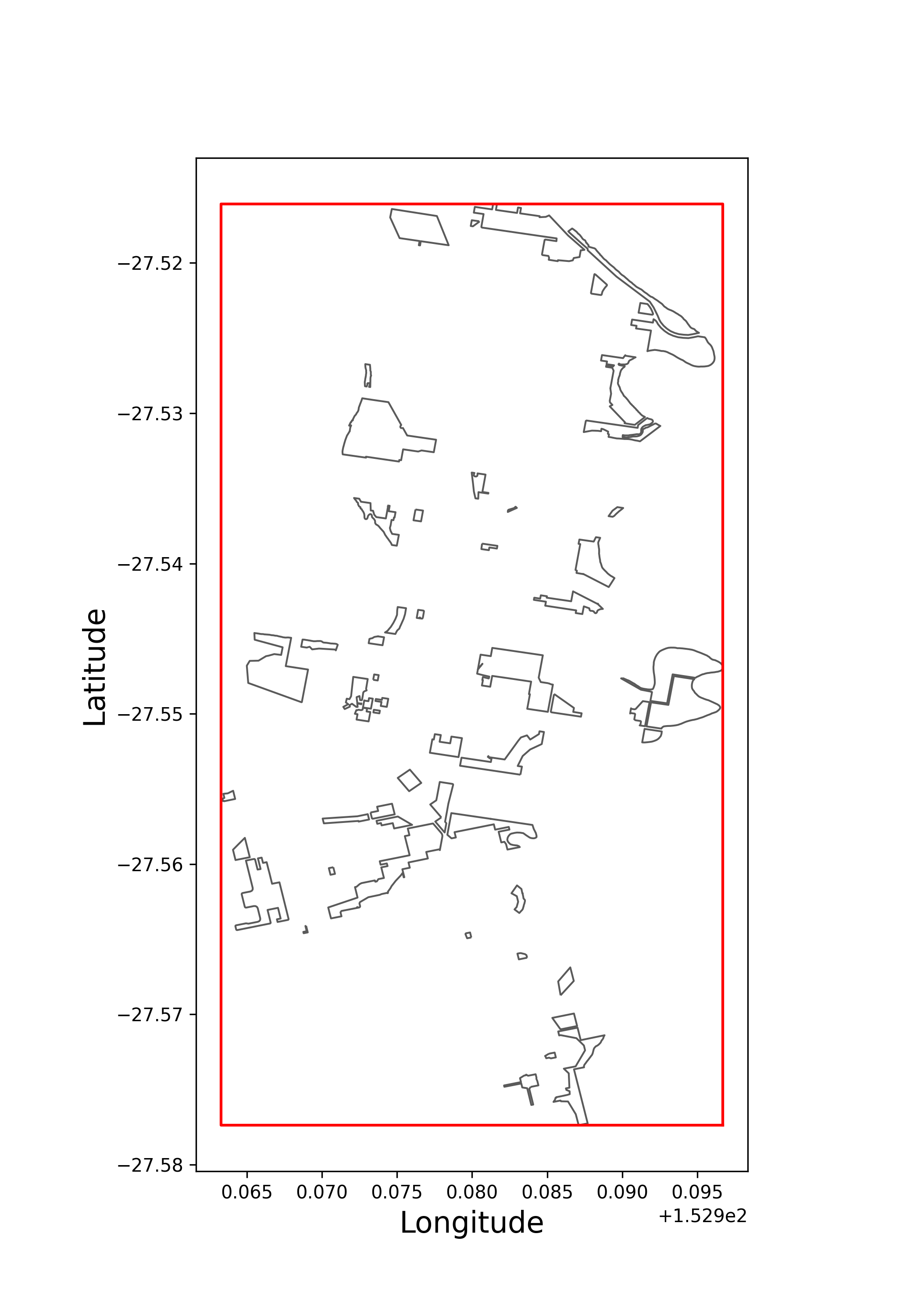
>>> # second, get a shape of all the Brisbane parks and draw a bounding box around it
>>> import shapely
>>> from shapely.ops import unary_union
>>> brisbane_parks_all = gpd.GeoSeries(unary_union(brisbane_parks["geometry"]))
>>> brisbane_parks_bbox = brisbane_parks_all.bounds
         minx       miny        maxx       maxy
0  152.963302 -27.577386  152.996692 -27.516073
To visualise
>>> plot_brisbane_parks_bbox = shapely.box(xmin=brisbane_parks_bbox["minx"][0],
...                                xmax=brisbane_parks_bbox["maxx"][0],
...                                ymin=brisbane_parks_bbox["miny"][0],
...                                ymax=brisbane_parks_bbox["maxy"][0]
...                                )
>>> brisbane_parks_all.plot(edgecolor = "#5A5A5A", linewidth = 1, facecolor = "white", figsize = (7,10))
>>> plt.plot(*plot_brisbane_parks_bbox.exterior.xy,color="red")
>>> plt.ylabel("Latitude",size=16,x=.45,y=0.5)
>>> plt.xlabel("Longitude",size=16)
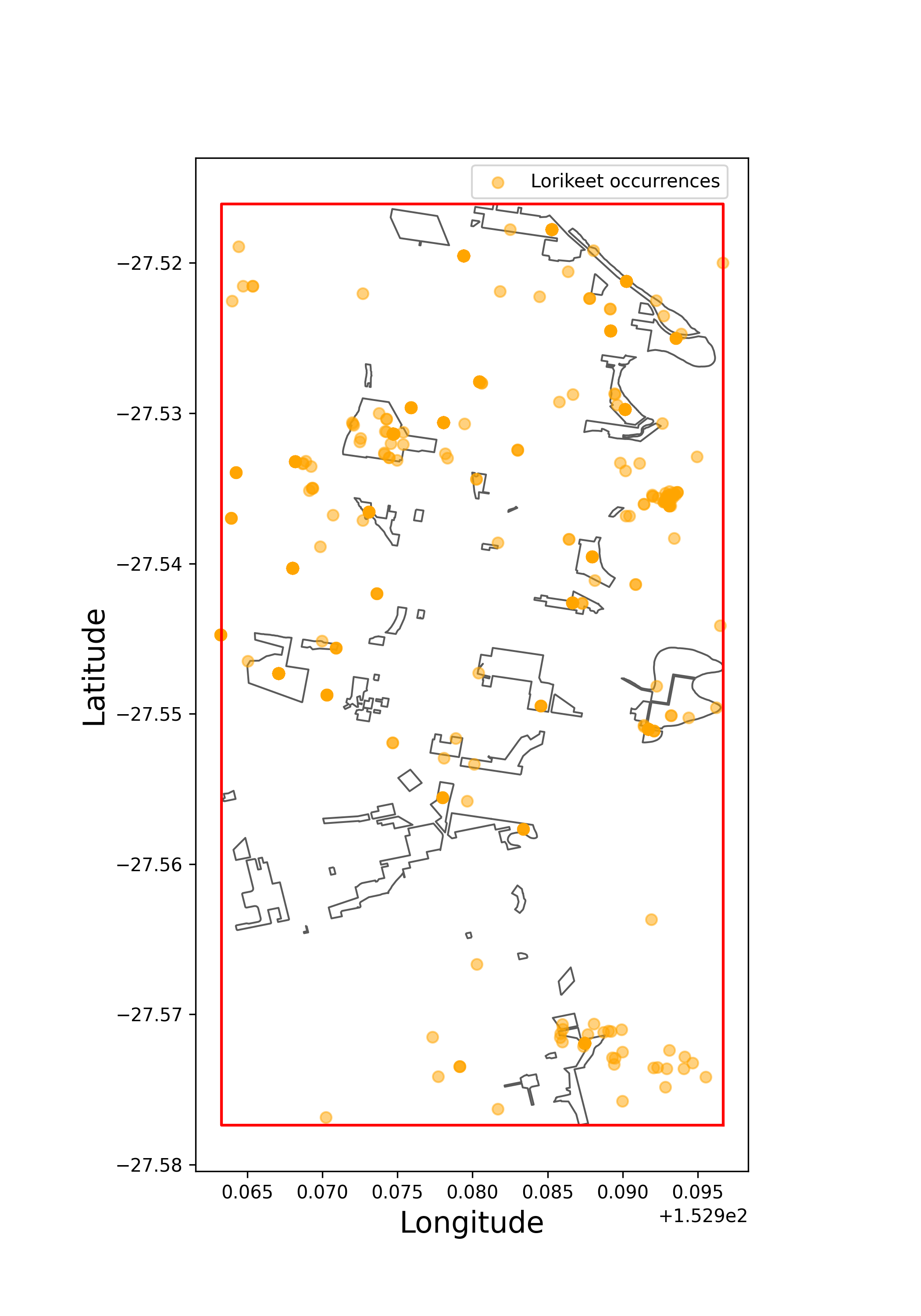
>>> # third, find all occurrences of Trichoglossus chlorolepidotus in the bounding box in 2022
>>> import galah
>>> galah.galah_config(email="your-email-here")
>>> lorikeet_brisbane = galah.atlas_occurrences(
...     taxa="Trichoglossus chlorolepidotus",
...     filters="year=2022",
...     bbox=brisbane_parks_bbox
... )
>>> lorikeet_brisbane
      decimalLatitude  ...  occurrenceStatus
0          -27.577001  ...           PRESENT
1          -27.576858  ...           PRESENT
2          -27.576303  ...           PRESENT
3          -27.576212  ...           PRESENT
4          -27.576212  ...           PRESENT
...               ...  ...               ...
3895       -27.517759  ...           PRESENT
3896       -27.517759  ...           PRESENT
3897       -27.517759  ...           PRESENT
3898       -27.517759  ...           PRESENT
3899       -27.517759  ...           PRESENT

[3900 rows x 8 columns]
>>> brisbane_parks_all.plot(edgecolor = "#5A5A5A", linewidth = 1, facecolor = "white", figsize = (7,10))
>>> plt.plot(*plot_brisbane_parks_bbox.exterior.xy,color="red")
>>> plt.ylabel("Latitude",size=16,x=.45,y=0.5)
>>> plt.xlabel("Longitude",size=16)
>>> plt.scatter(lorikeet_brisbane["decimalLongitude"],lorikeet_brisbane["decimalLatitude"],alpha=0.5,color="orange",label="Lorikeet occurrences")
>>> plt.legend(loc=(0.5,0.96))
>>> # Filter records down to only those in the shapefile polygons
>>> brisbane_parks["count"] = pd.Series([0 for i in range(len(brisbane_parks))])
>>> for i,park in brisbane_parks.iterrows():
...     points = [(x,y) for x,y in zip(lorikeet_brisbane["decimalLongitude"], lorikeet_brisbane["decimalLatitude"]) if shapely.contains_xy(park["geometry"],x,y)]
...     brisbane_parks.at[i,"count"] = len(points)
>>> brisbane_parks_counts = brisbane_parks[["PARK_NAME","count"]].sort_values("count",ascending=False).reset_index(drop=True)
>>> brisbane_parks_counts.head(10)
                        PARK_NAME  count
0                NYUNDARE-BA PARK    846
1              SHERWOOD ARBORETUM    706
2                   FAULKNER PARK     65
3              FORT ROAD BUSHLAND     55
4               BENARRAWA RESERVE     48
5         STRICKLAND TERRACE PARK     48
6  GRACEVILLE RIVERSIDE PARKLANDS     34
7                  NOSWORTHY PARK     22
8           HORACE WINDOW RESERVE     16
9          GRACEVILLE AVENUE PARK      9
Some shapefiles cover large geographic areas with the caveat that even the bounding box doesn’t restrict the number of records to a value that can be downloaded easily. In this case, we recommend more nuances and detailed methods that can be performed using looping techniques. One of our ALA Labs blog posts, Hex maps for species occurrence data, has been written detailing how to approach larger problems such as this.